Why Your AI Factory Is Secretly a Dynamical System (And 5 Other Counter-Intuitive Truths About Modern AI Inference)

System overview

Floor: Electrical distribution, liquid and air cooling, HBM, and interconnect. These are not decorations around the model. They set the feasible compute.

Serving stack: Gateway, router, batcher, engine. They turn request shape into queue depth, batch mix, and KV leases.

Clients: Timeouts, retries, backoff, and multi-turn agents. They write the next arrival process from the last latency.

Telemetry: GPU utilization, mean load, rack power. Useful signals. Dangerous if you treat each one as the plant.

The cross-layer chain I keep seeing is:

The state at time $t$ is not a list of independent numbers. It is a heterogeneous vector

$$x_t = (x_{\mathrm{phys}}, x_{\mathrm{comp}}, x_{\mathrm{net}}, x_{\mathrm{serv}}, G_t)$$

that couples thermals, clocks, queues, and a variable-sized memory graph.

AI inference infrastructure is increasingly a physical computational system rather than a collection of servers running software.

What I observed

Teams still operate these plants as if isolated metrics were enough. Aggregate GPU compute utilization. Average server load. Overall rack power. The dashboard stays green while a localized thermal spike or a power-cap cut walks up the stack and lands as a queue, a worse batch mix, and a missed TTFT.

I have already written the 62% GPU utilization OOM. That weekend was not a freak dashboard bug. It was the memory-headroom paradox in production: compute occupancy said there was room, the allocator said there was not.

The same mistake shows up in load. Two traces with a 50 requests/second mean can have totally different queues. And it shows up in clients. When TTFT rises, retries write a new demand process. The original spike can be gone and the plant stays full.

Why I think this happened

Single-variable telemetry creates an illusion of control. It cannot see the feedback loops. A physical event at one layer changes frequency, capacity, queue, batch, and SLO. If you only watch one layer, you will scale, cap, or retry the wrong thing.

To operate under energy and physical bounds, the plant has to be treated as a dynamical system. You estimate state, you model how fast and slow clocks interlock, and you evaluate interventions before you throw a lever.

Finding 1: The GPU is not full, but the system is crashing

Claim. Moderate GPU utilization does not imply allocatable memory. Utilization $\nRightarrow$ available computational capacity.

Evidence. An OOM can fire while telemetry reports about 62% GPU compute utilization. I reconstructed one of those weekends in Why Agent Workloads OOM at 62% GPU Utilization. Seven of twelve replicas died. nvidia-smi still looked relaxed.

Explanation. $U_{\mathrm{GPU}}$ measures SM occupancy in a sampling window. It says nothing about whether the next KV block can be placed. In LLM serving, HBM is eaten by dynamic KV, prompt fragmentation, batching policy, and long context.

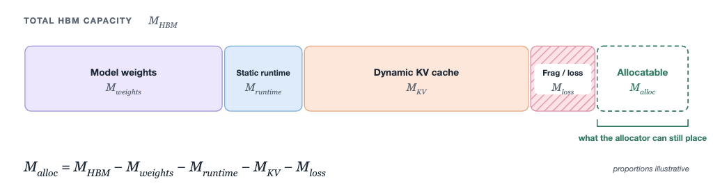
At evaluation time $t$:

$$M_{\mathrm{alloc}} = M_{\mathrm{HBM}} - M_{\mathrm{weights}} - M_{\mathrm{runtime}} - M_{\mathrm{KV}} - M_{\mathrm{loss}}$$

$M_{\mathrm{loss}}$ is request-dependent allocation loss and external fragmentation. Track it explicitly. Do not double-count blocks already in the measured allocations.

Because KV scales with sequence length, concurrency, and agent turns, $M_{\mathrm{alloc}}$ can hit zero while $U_{\mathrm{GPU}}$ stays moderate. When $M_{\mathrm{alloc}} \to 0$, the allocator fails. That is an OOM with “spare” compute.

Implication. Page on allocatable KV headroom and fragmentation, not on SM busy.

Finding 2: Average load is a lie

Claim. Same mean demand $\nRightarrow$ same trajectory.

Evidence. A bursty arrival trace and a steady trace can share the same mean (say 50 requests/second) and produce different queue depths, tail latency, and failure profiles.

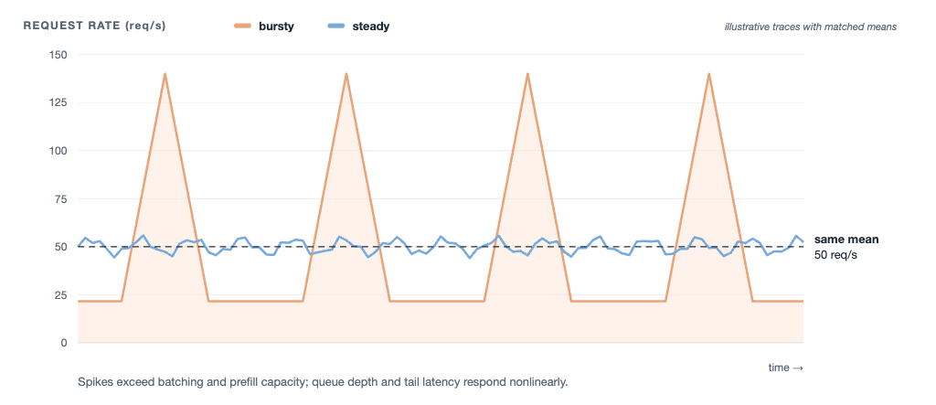
Explanation. Point-in-time averages hide spikes that exceed batching and prefill capacity. Prefill is compute-bound. Decode is memory-bandwidth-bound. They react differently to the same transient. Latency grows nonlinearly with queue depth, so a bursty trace violates tails that a steady stream with the same mean never sees.

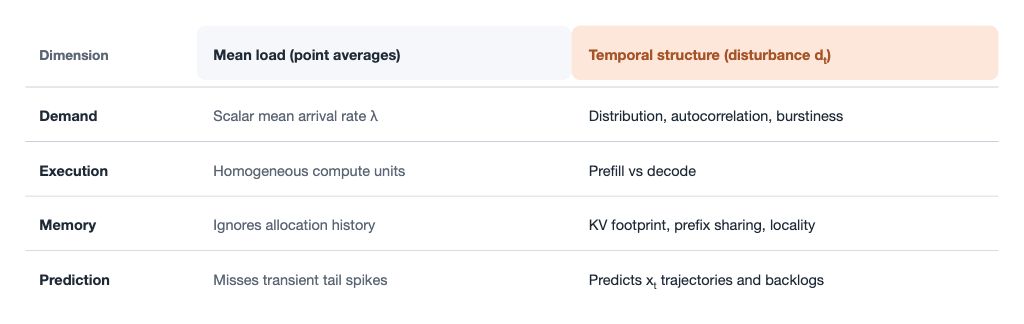
A compressed history $w_t = \psi(d_{t-L:t})$, or a summary $s(d_{0:t})$, is sufficient only if the future state over horizon $H$, given that summary, matches the future given the full disturbance history:

$$p(x_{t+1:t+H} \mid s(d_{0:t}), \hat{x}_t, a_{t:t+H}) \approx p(x_{t+1:t+H} \mid d_{0:t}, \hat{x}_t, a_{t:t+H})$$

High autocorrelation, variable context lengths, or temporal concentration fail that test. Rate-only metrics then hide the queue you are about to grow.

Implication. Capacity-plan on traces and phase mix, not on a mean QPS slide.

Finding 3: Demand is not external

Claim. Under high TTFT, realized arrivals are a function of your own latency. Retry storms can keep a system overloaded after the trigger is gone. That is a metastable failure.

Evidence. Classical open-loop design treats $d_t$ as exogenous. In serving, timeouts, retries, backoff, and multi-turn agent loops generate extra arrivals when the queue is already long.

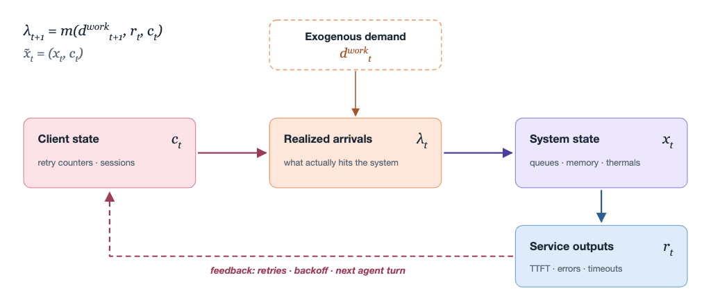
Explanation. Exogenous intent $\xi_{t+1}$ is not the same as realized arrivals $a_{t+1}$. Realized demand depends on past outcomes $y_t$ and client state $c_t$:

$$a_{t+1} = g(\xi_{t+1}, y_t, c_t)$$

When $y_t$ triggers retries, $c_t$ joins the plant. The augmented state is $\tilde{x}_t = (x_t, c_t)$. The facility can sit in retry-induced persistent overload: saturated and unusable after $\xi_t$ has cleared.

Implication. Model clients as part of the plant. Cap retries and admission before you add replicas to serve your own timeouts.

Finding 4: One clock cannot run the data center

Claim. A single global $\Delta t$ either averages away kernel dynamics or freezes thermal state.

Evidence. The same facility has phenomena on microseconds, milliseconds, and seconds-to-minutes.

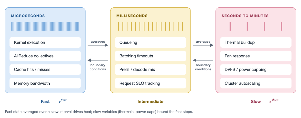
1. Microseconds: kernel launches, tensor-parallel AllReduce, memory-bus transactions, L1/L2 hits and misses.
2. Milliseconds: queues, batching timeouts, prefill/decode steps, request-level SLO clocks.
3. Seconds to minutes: thermal buildup, cooling response, DVFS power caps, node autoscaling.

Explanation. Fast dynamics (index $k$, milliseconds) and slow dynamics (index $j$, seconds) interlock:

$$x^f_{k+1} = f_f(x^f_k, a^f_k, d_k; x^s_j)$$ $$x^s_{j+1} = f_s(x^s_j, \bar{x}^f_j, a^s_j)$$

Slow variables (thermals, power caps) are boundary conditions for fast steps. The fast state averaged over a slow interval, $\bar{x}^f_j$, drives heat. Under singular perturbation, fast states sit on a quasi-steady manifold of the slow boundaries:

$$\varepsilon\,\dot{x}_f = g(x_f, x_s, a, d), \quad \varepsilon \ll 1, \quad x_f \approx x_f^*(x_s, a, d)$$

Implication. Do not sample the plant at one rate and call it a twin. Keep the clocks, then couple them.

Finding 5: Forecasting is not intervening

Claim. Prediction ≠ intervention. A model trained on observed actions is not a model of what happens if you force a new action.

Evidence. Passive forecasting computes

$$p(r_{t+k} \mid o_{0:t}, a_{0:t})$$

That is the next reading if the old policy continues. Control needs the outcome of an intervention, with future disturbances $d_{t:t+k}$ and hardware structure $\theta$ held in view:

$$p\!\left(r_{t+k} \mid \mathit{do}(a_{t:t+k} = a^*_{t:t+k}), o_{0:t}, d_{t:t+k}, \theta\right)$$

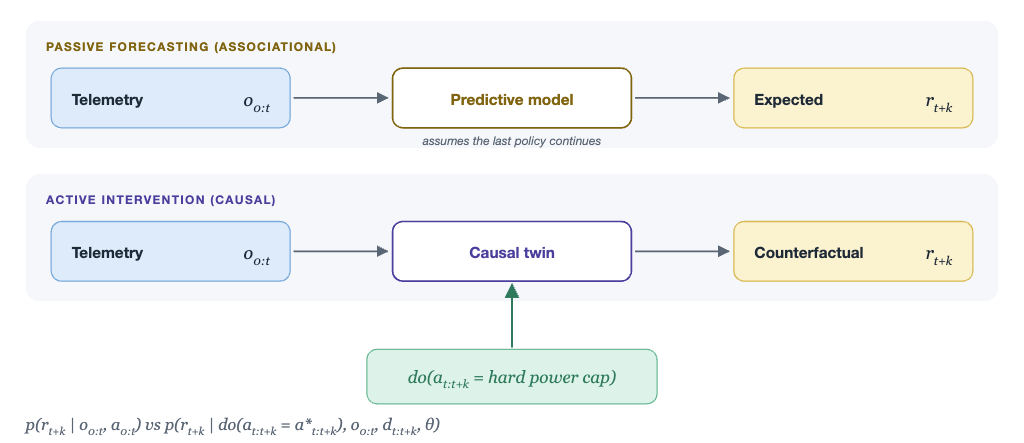
Explanation. Observational models correlate history under past operating policy. Impose a hard power cap ($\Delta a_{\mathrm{power}} < 0$), change batch bounds, or reroute traffic, and the joint distribution moves. The fit breaks.

The plant is also not one smooth $f$. It switches regimes $z_t \in \{\text{Normal}, \text{Saturated}, \text{Thermal-constrained}, \text{Power-capped}\}$:

$$x_{t+1} = f_{z_t}(x_t, a_t, d_t; \theta) + \varepsilon_t$$

A digital twin that cannot switch regimes cannot evaluate $\mathit{do}(a_{t:t+k})$ before you touch live hardware. Identifying an intervention effect needs assumptions beyond an associational fit. That is Pearl’s structural causal framework, not a nicer RMSE.

Implication. Do not drive power caps, batch limits, or routing from a forecast trained on the last policy. Evaluate $\mathit{do}(\cdot)$ first.

Finding 6: System state is trees and graphs

Claim. Serving state is not only $x_t \in \mathbb{R}^n$. Autoregressive serving stores structure.

Evidence. Prefix sharing, tree-shaped prompt execution (RadixAttention), and paged KV (PagedAttention) make $G_t$ part of the state.

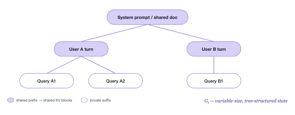
Explanation. A scalar “free bytes” number loses prefix-sharing ratio, cache locality, and recomputation cost. To collapse $G_t$ to a summary $\psi(G_t) \in \mathbb{R}^k$, the map has to be sufficient over horizon $H$:

$$p(x_{t+1:t+H} \mid z_t, \psi(G_t)) \approx p(x_{t+1:t+H} \mid z_t, G_t)$$

That means occupancy, prefix-sharing ratios, reuse-distance quantiles (p50/p90), and eviction rates. If $\psi$ loses those, you will predict free memory and still miss a recompute storm.

Implication. Treat the prefix tree as first-class state, the way a cluster KV directory is first-class in Why KV Cache Needs a Directory.

The mental model

The plant is one regime-switching dynamical system:

$$x_{t+1} = f_{z_t}(x_t, a_t, d_t; \theta) + \varepsilon_t \quad \text{(latent state)}$$ $$o_t = h(x_t; \theta) + \nu_t \quad \text{(partial telemetry)}$$ $$r_t = g(x_t, a_t, d_t; \theta) + \xi_t \quad \text{(service and energy outcomes)}$$

An operational AI-factory digital twin does four jobs: infer latent state $\hat{x}_t$, update on more than one timescale, model closed-loop demand, and evaluate structural interventions $\mathit{do}(a_t)$ before they hit the floor.

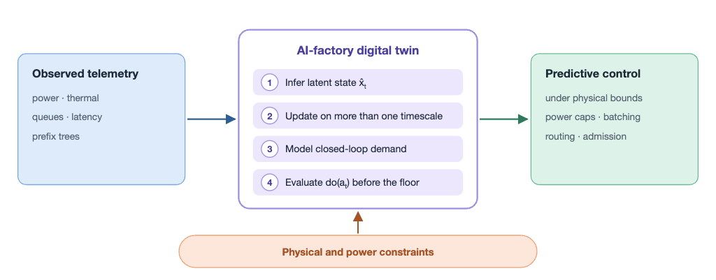
Joule exists because tokens, watts, and SLOs are the same ledger. A twin that cannot see power as a constraint will optimize the wrong objective.

Practical guidance

1. Watch the chain, not one gauge. Power and thermal events should show up as queue, batch mix, and TTFT, not only as rack watts.
2. Alert on $M_{\mathrm{alloc}}$ and KV leases. 62% GPU utilization is compatible with an OOM.
3. Keep arrival traces. Mean QPS is not a workload.
4. Put retry counters in the state. Admission-control the storm you are causing.
5. Sample fast and slow clocks separately, then couple them.
6. Test $\mathit{do}(\mathit{power\_cap})$, $\mathit{do}(\mathit{batch\_bound})$, and $\mathit{do}(\mathit{route})$ on a twin that can switch regimes.
7. Summarize prefix trees with sharing and reuse, not only free bytes.

Limitations

This is a systems argument and a field synthesis, not a controlled A/B on a named model and SKU. The 62% OOM and the queueing claims reuse measurements I have already published. The 50 requests/second traces are a pedagogical pair with a shared mean, not a claim about one customer. Sufficiency, multi-rate, and do-calculus statements are modeling conditions. They hold only under the independence and regime assumptions you are willing to state. Results will differ across engines (vLLM, SGLang, TensorRT-LLM), disaggregated prefill/decode, and how aggressively the runtime shares prefixes.

The open question

As regional grids, thermal envelopes, and electrical plant become the ceiling, how should hardware-software co-design change when a grid power cap, not spare silicon, is the hard constraint on AI capability?

@article{abi2026aifactorydynamicalsystem,
  title = "Why Your AI Factory Is Secretly a Dynamical System (And 5 Other Counter-Intuitive Truths About Modern AI Inference)",
  author = "Aryan, Abi",
  journal = "abiaryan.com",
  year = "2026",
  month = "October",
  url = "https://abiaryan.com/writing/ai-factory-dynamical-system/"
}