Problems and Challenges in AutoML

March 16, 2019

^{Article based on the research paper Problems & Challenges in AutoML, 2019. I would like to thank my co-author Shubhi Sareen for being an excellent research collaborator through this research.}

The constantly growing amount and complexity of data involved in brain studies makes manual parameterization of data processing and modelling algorithms a tedious and time-consuming task. One of the key focuses for the machine learning community has been to develop autonomous agents, by automating the entire production pipeline for selecting and training the learning algorithms, so as to take humans out of the loop. This automation has several benefits including reducing human effort and the associated time cost involved, improving the performance of these algorithms by tailoring them to the problem at hand, reducing human induced bias as well as improving the improving the reproducibility and fairness of the scientific studie s. In this paper, we will be discussing some of the key problems and challenges in AutoML. Our survey will cover central algorithms in AutoML including NAS, etc. In parallel, we also highlight the unique advantages of deep neural network, focusing on developing algorithms that can generalize of different tasks via AutoML. To conclude, we describe several current areas of research within the field.

While neural networks were not the first choice for designing machine intelligence, it was in 2012 that neural networks began outperforming competing techniques for tasks that required complex feature engineering [Hinton, Sutskever 2012]. This advent of deep learning has had a significant impact on many areas in machine learning, dramatically improving the state-of-the-art in tasks such as object detection, speech recognition, and language translation.

Why Deep Learning for AutoML?¶

While AutoML is not simply limited to deep learning methods, classical machine learning becomes limited by the need for simpler rules and features. The key foundation for deep learning is compositionality, which means it is possible to construct a task from a series of sub-tasks.

For most of the tasks we can divide them into two categories - classification problems and regression problems. Deep Learning has shown excellent promise on classification problems. And one could argue that one of the key contributors for this success on classification problem is the convolutional neural networks.

Convolutional Neural Networks consist of multiple layers and are designed to require relatively little pre-processing compared to other classification algorithms. They learn by using filters and applying them to the images. The algorithm takes a small square (or ‘window’) and starts applying it over the image. This mathematical process is called convolution. Each filter allows the CNN to identify certain patterns in the image. The CNN looks for parts of the image where a filter matches the contents of the image. The first few layers of the network may detect simple features like lines, circles, edges. In each layer, the network is able to combine these findings and continually learn more complex concepts as we go deeper and deeper into the layers of the Neural Network. Thus, deep learning essentially allows us to map complex features from inputs to a classification.

For this complex feature engineering, the number of available choices of algorithms, learning methods and packages for machine learning have quadrupled in the past decade. The algorithm choice space ranges from CNNs, LSTMs to GANs. Learning methods ranging from K-means clustering, PCA (Principal Component Analysis), Bayesian Optimization to Q-Learning. The number of packages ranging from Tensorflow, Scikit-Learn, PyTorch, etc.

When doing AutoML these days, the performance is hugely dependent on the design decision of the model. These design decisions include - algorithm selection and hyperparameter optimization. Usually, this optimization process for any selected algorithm is repeated via hit and trial until we find a good set of choices for each dataset. This problem has been dubbed as CASH (Combined Algorithm Selection and Hyperparameter Optimization) and can present a combinatorial number of choices for any user. For any non-expert, this often results in choosing an algorithm based on either reputation or intuitive appeal and more often than not, leaving the hyperparameter settings to default thus resulting in less than optimal performance for that particular selection of models. Lately, Tensorflow has helped make this process slightly easier by allowing the users a visual representation of the process and an almost plug and play like interface for optimization settings, however the choice of algorithm selection and learning method selection is still heavily user-dependent.

History¶

The goal of AutoML is largely to build autonomous agents that can take human out of the loop for choosing and designing learning algorithms. This can potentially mean huge gains in the performance of machine learning algorithms by tailoring them to the problem at hand, reducing human induced bias as well as improving the improving the reproducibility and fairness of the scientific studies.

We roughly divide this section in two parts-

the Model Selection where we discuss the problem of architecture design (also known as Search Space) and Learning Policy Selection, and
Model Optimization where we discuss the problem of optimization choices made while training the model including hyperparameters, ensembles and regularizers. In this section, we will go through the reasoning behind some of these decisions.

For image classification, various architectures have been proposed over the years. The convolution neural network architecture was first proposed in LeNet-5, which consisted of 6 layers consisting of convolution, average pooling and hidden layers. However, because of low computational resources, convolutional architectures next came into attention in 2012 with the first fast implementation of CNNs on GPU, AlexNet. AlexNet employed 8 layers, including 5 convolutional and 3 fully connected layers using the ReLU activation function. The authors highlighted the gains in performance using ReLU over tanh and sigmoid activation functions. Dropout was used in the fully connected layers to prevent overfitting.

In 2014, VGGNet was proposed which consists of 16 convolution and three fully connected layers employing only 3x3 convolutions. Next, GoogleNet was proposed which consisted of 22 layers. The main intuition behind the model was to make it compatible to be used on a smartphone with 12 times lesser parameters than AlexNet. It employed inception modules, which convolve parallely using different sizes of filters. Next, in 2015, ResNet was proposed which introduced skip-connections between the layers. These skip connections allowed a 152 layer architecture to be trained, while still having complexity lesser than that of VGGNet.

Thus the advances in image classifications can be attributed to two main features-

Increasing the number of layers
Introduction of operations/connections which reduces the amount of parameters to be trained.

However, the process of defining the number of layers is still controlled majorly by human beings and the hyperparameters are hand-tuned, therefore requiring a lot of time to be invested. The next step was to model these techniques automatically, thereby leading to the introduction of AutoML.

What is AutoML?¶

To define the problem of AutoML,

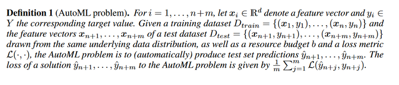
In the past five years, various AutoML methods have been proposed. Introduced in 2013, Auto-WEKA was the first AutoML method and used Bayesian Optimization to automatically instantiate a highly parametric machine learning framework. Parametric models assume some finite set of parameters $\theta$. Given the parameters $\theta$, future predictions, x, are independent of the observed data, D

\[ P(x|\theta, D) = P(x|\theta) \]

It is based upon the assumption that $\theta$ captures everything there is to know about the data and thus the complexity of the model is bounded even if the amount of data is unbounded.

While these parametric methods are simpler, faster, interpretable and can be trained with less data but they pose flexibility constraints while struggling with complex data generating a poor fit for the real world problems. It was further extended as a package called Hyperopt-sklearn in 2014 to non-parametric methods like probability calibration, density estimation provided by Scikit-Learn. One of the key achievements of Hyperopt-sklearn is an ability to remove redundant features, or reduce data dimensionality using SVM or PCA so the classification task can become simpler.

While one possible direction post this could be extending the framework to support more machine learning algorithms or extending the number of pre-processing methods however the ability to select a good algorithm and a combination of the right hyperparameters is a problem that lies at the heart of AutoML.

Introduced in 2015, Auto-sklearn approached the problem by taking into account past performance on similar datasets, or constructing ensembles from the models evaluated during the optimization. While budget and computational power being the obvious constraints for such methods, one not-so-obvious limitation is that testing hundreds of hyperparameter optimization configuration increases the risk of overfitting to the validation set.

Aside from this, several incremental developments have been made in the field of architecture selection, hyperparameter optimization and meta-learning using both gradient based as well as gradient-free methods.

Gradient Free Techniques¶

The most intuitive gradient-free technique is random search i.e. randomly searching the state-space domain to find optimal values. However, since the state space is multi-dimensional, therefore, leading to suboptimal results using random search. Population based methods such as Genetic Algorithms and Particle Swarm Optimization have been employed in order to search the state-space more effectively. Other gradient free techniques include Bayesian Optimization by modelling the loss of a configuration, where the improvement of a configuration is proportional to the distance between the best-so-far loss and the predicted mean or using Tree Based Estimator like MCTS or using surrogate models for instance Gaussian processes. Q-learning has also been used in order to learn desirable architectures, where a reinforcement agent chooses components of an architecture sequentially with the reward equal to the validation accuracy.

Gradient Based Techniques¶

In the past few years, deep learning methods have shown immense potential in the area of AutoML. One such key project is Auto-Net which uses Bayesian Optimization method SMAC and the deep learning library Lasagne, later followed by Auto-Net 2.0 that uses a combination of Bayesian Optimization and HyperBand, called BHOB, and uses PyTorch as the key deep learning library. Auto-Net provides automatically-tuned feed-forward neural networks without any human intervention. BHOB uses repeated runs of successive halving to invest most runtime in promising neural networks and stops training neural networks with poor performance early and using kernel density estimator to describe regions of high performance in the space of neural network. One of its key advantages is that this method is highly parallelizable achieving almost linear speedups with an increasing number of workers. Auto-Net performance on three different datasets -

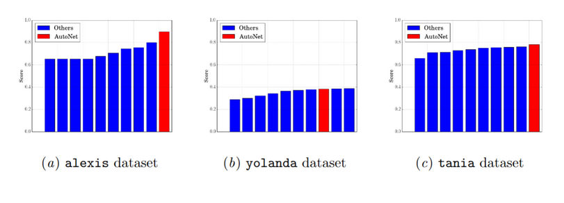
As observed, AutoNet performs best twice and comparatively well for yolanda as well. As the No Free Lunch theorem goes, any one algorithm that searches for an optimal cost or fitness solution is not universally superior to any other algorithm given that we are optimizing for fit on a limited class of problems thus it may or may not generalize in an infinite possibilities dataset. Thus gradient based neural networks started to focus on building a model from existing class of models instead of random search on a particular number of configurations. In 2016, the focus shifted from searching within specified parameters to instead the use of modular approach to find the best model and combination of hyperparameters.

Model Selection - Architecture Design and Learning Policy Selection¶

In 2016, MetaQNN was introduced to generate CNN Architectures for a given task using Q-Learning, where the agent chooses the architecture layers sequentially, via the epsilon-greedy strategy, with reward equal to the validation accuracy. Next, the problem of generating a high-performing architecture was dealt by using a meta-controller. A meta controller models state information and directs how the search space is to be navigated in order to find the optimal architecture. Traditionally, RNNs and LSTMs are used as metacontrollers, encoding the state space information. The state space consists of various blocks performing operations like convolution and pooling, and the meta-controller, say RNN, arranges these blocks in an end-to-end fashion. The controller is then updated based upon the validation accuracies to produce a better performing architecture in the next iterations.

Another new approach in 2016, was the creation of NAS. The intuition behind this was since a single model does not generalize well for different datasets. Let’s try to automate the process of building a system that can adapt to different datasets. This was done by using smaller pieces from the architecture to build a new architecture using a technique called convolutional cells. However, limitations of this approach are it does limit itself to using the same type of controller and same kind of model for every image, which might or might not be optimal. Also, it happens to be computationally expensive. Progressive Nets however were the next iteration. Progressive Nets employ sequential-based model optimization to further optimize the search process. It learns the architecture in increasing complexity, with first learning the cell structure and then stacking those together to form a CNN.

The next in line was ENAS i..e efficient neural architecture search. In 2017, Efficient Architecture Search was proposed to reuse the weights of pre-existing architectures using a Reinforcement Agent as a meta-controller. The architecture is encoded into a low dimensional representation using a bidirectional RNN with Embedding Layer. The network transformations are produced by an independent actor network which takes in as input the encoded representation. Efficient Neural Architecture Search is the next step to reduce the dependence on computational resources for generating high performance architectures. A policy gradient approach is used to train a controller which can select optimal subgraphs from within a larger graph. It allows the children graphs to share weights, therefore allowing faster convergence. ENAS employs LSTM as a controller. The training procedure consists of alternating between learning the parameters shared by the children and that of the LSTM controller.

In addition to the requirement of high computational costs, the performance of network architectures learnt on a specific dataset don’t transfer to other tasks. In order to overcome that, in BlockQNN the authors proposed to generate the architecture block-wise, rather than layer-wise. The optimal block structure is searched using Q-Learning with $\epsilon$-greedy strategy and experience relay. Lately, there has been a influx of various AutoML methods like Elastic Architecture Transfer for Accelerating Large-scale Neural Architecture Search (EAT-NAS), Graph HyperNetworks for Neural Architecture Search, Stochastic Neural Architecture Search (SNAS), Instance-aware Neural Architecture Search (Insta-NAS) etc that use several approaches that we will discuss in further sections.

One of the major drawbacks of these approaches is the fact that each architecture is trained from scratch, thereby basing their success on external factors like availability of computational resources. However, In the limited computational resource scenario, Bayesian Optimization techniques have emerged to be very successful for their ability to work with combinatorial space problems with limited training time as well as their flexibility with high-dimensional problems and transfer learning problems.

Architecture Search via Bayesian Optimization¶

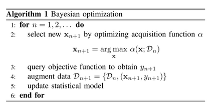
Bayesian optimization has emerged as an exciting subfield of machine learning that is concerned with the global optimization of noisy, black-box functions using probabilistic methods. Essentially, Bayesian Optimization is a sequential model-based approach to machine learning.

Mathematically, the problem of finding a global maximizer (or minimizer) of an unknown objective function f can be represented as

x* = arg max f(x) for x in X’ where X’ is some design space of interest.

One of the key advantages of Bayesian Optimization framework is that it can be applied to unusual search spaces that involve conditional or categorical inputs, or even combinatorial search spaces with multiple categorical inputs. The Bayesian Optimization framework has two key ingredients - first, a probabilistic surrogate model which consists of a prior distribution that captures our beliefs about the behaviour of the unknown objective function and an observation model that describes the data generation mechanism and secondly, the loss function that describes how optimal a sequence of queries are. In practice, these loss functions are often expresses as a form of regret, either simply or cumulative which is then minimized to select an optimal sequence of queries.

If f is cheap to evaluate we could sample at many points e.g. via grid search, random search or numeric gradient estimation. However, if function evaluation is expensive e.g. tuning hyperparameters of a deep neural network, probe drilling for oil at given geographic coordinates or evaluating the effectiveness of a drug candidate taken from a chemical search space then it is important to minimize the number of samples drawn from the black box function f. This is the domain where Bayesian optimization techniques are most useful. They attempt to find the global optimum in a minimum number of steps. A popular surrogate model for Bayesian optimization are Gaussian processes (GPs). The success of these methods has led to the discovery and development of several acquisition functions including Thompson Sampling, Probability of Improvement, Expected Improvement, Upper Confidence Bounds, Entropy Search etc. These acquisition functions trade off exploration and exploitation such that their optima is located where the uncertainty in the surrogate model is large (exploration) and/or the prediction is high (exploitation).

In terms of AutoML, it has been proved through various experiments that often the careful choice of statistical model is often far more important than the choice of acquisition functions. While Bayesian Optimization is already one of the preferred methods for combinatorial search spaces and policy search for both parametric as well as non-parametric models, one of the major applications in AutoML has been the exploration of Bayesian Optimization for Automating Hyperparameter Tuning. In architectural search spaces, Bayesian Optimization methods have received great attention in tuning deep belief networks, Markov Chain Monte Carlo Methods (MCMC), Convolutional Neural Networks and its application in one of the most primitive neural architecture search methods such as SMAC, Auto-SkLearn, AutoWeka, BHOB, REMBO etc.

Another key application of Bayesian Optimization has been on multi-task learning and transfer learning, esp in a constrained budget. There have been several attempts to exploit this property within the Bayesian Optimization framework including Collaborative Hyperparameter Tuning, Initializing Bayesian Hyperparameter Optimization via Meta-Learning, Sequential Model-Based Optimization for General Algorithm Configuration, Gaussian Process Bandit Optimization, Freeze-Thaw Optimization, Efficient Transfer Learning via Bayesian Optimization. The key idea here is that there are several correlated functions, $\tau$ = {1, 2, ….,M}, called tasks and that we are interested in optimizing some subset of these tasks, thus using the data from one task to provide information about another task.

One such method of sharing information between tasks has been implementing by modifying the Bayesian Optimization Routine to modify the underlying the Gaussian Process (GP) model called Multi-Output GPs. We define a valid covariance over input and task pairs, k((x,m), (x’, m’)). One of the explored methods to do this is using coregionalization that utilizes the product kernel -

\[ k((x,m), (x’, m’)) = k_{\chi}(x,x')k_{\tau}(m,m') \]

Where m, m’ $\in$ $\tau$ . The problem of defining a Multi-Output GP can then be viewed as learning a latent function, or a set of latent functions, that can be transformed to produce the output tasks. This can be done by introducing a latent ranking function across different pairs of observations on various tasks such that the tasks are jointly embedded in a single latent space that in variant to potentially different output scales across tasks. The key idea here is to build a joint model with a joint probability distribution function which can then be trained via various methods like Random Forest to learn the similarities between different tasks based on the task features. The best inputs from the most familiar tasks (or models) are then used as the initial design for the new task (or new model) thus creating an automatic architecture space pipeline for working on cross domain machine learning models.

Architecture Search via Evolutionary Methods¶

An evolutionary algorithm based approach is used to evolve AmoebaNet-A, an architecture for image classification at par with human crafted designs. The proposed approach biases tournament selection with age, thereby preferring younger genomes. The search space consists of directed graphs where hidden states correspond to vertices and ordinary operations like convolution, pooling etc. are associated with edges. Mutation is performed either by random reconnection of edges to other vertices or relabeling randomly selected edges. After initializing the parent population with randomly generated architectures which are trained and evaluated, children architectures are generated using mutation. These architectures are then trained and evaluated, whereas the oldest ones are discarded. The ageing evolution used is analogous to regularization, as the only way good architectures can be retained are when they are inherited by the children. Since at each step, children models are retrained, architectures which constantly perform good, are the ones which are eventually retained, thereby preventing overfitting.

In GeneticCNN, Genetic Algorithms are used to come up with Convolutional Neural Network Architectures. A binary string is used to represent each possible network. 0.5 $\Sigma$ sKs(Ks-1) bits are needed to represent the network with S stages, and each stage having Ks nodes. The bit corresponding to (vs,i, vs,j) is set if there is a connection between the associated nodes. A default input and output node are present at every stage. Isolated nodes do not have a connection to the default nodes. In case of absence of connections at a stage, i.e. all bits are unset, convolution is applied only once. Only convolution and pooling operations are taken into consideration. The initial population consists of randomized strings, where each bit is sampled from Bernoulli Distribution. Individuals are selected using Russian roulette process, where fittest individual has maximum probability of being selected. In mutation, a randomly selected bit is flipped with mutation probability. In crossover between two individuals, corresponding stage pairs are exchanged with crossover probability. Fitness is obtained by training the architectures represented by individuals on a preselected reference dataset.

Cartesian Genetic Programming is used to design architecture for Convolutional Neural Network which provides the benefit of flexibility to incorporate skip connections and variable depth networks in the representation. The network is defined as a directed acyclic graph represented using s two dimensional grid consisting of computational vertices. For a grid of Nr rows and Nc columns with fixed number of inputs and outputs, nodes in the nth column have connections from nodes in the range of (n-l) to (n-1) columns. The architecture representation in the genotype have fixed length integers, each chromosome consisting of type and connectivity information regarding that node. The phenotype consists of variable number of nodes because all nodes don’t have a connection to the output. Computational nodes comprises of convolution operation, average pooling, max pooling, summation, concatenation and ResBlock (convolution processing, batch normalization, ReLU, and tensor summation). A (1+ $\lambda$) evolution strategy is used to find the appropropriate architecture where the most fit of the $\lambda$ children generated at each generation become the parents for the next generation. Children architectures are trained in parallel and fitness is defined as the validation accuracy. The mutation strategy used is to change the type (size and number of filters) or the edge connections at random depending upon the mutation probability. In case of stagnation in fitness of children, mutation is applied to the non functioning nodes in the parent architectures. The proposed approach has an inherent drawback of high computational cost.

Another work analyzed the performance of gradient-free Genetic Algorithms on Reinforcement Learning Problems. The population of N individuals comprise of vector parameters for neural networks denoted by $\theta$i. On evaluating $\theta$i in every generation, a fitness score F($\theta$i) is associated with each individual which is analogous to reward. The most fit individuals become the parents in the next generation. Mutation is performed on randomly selected parent by addition of Gaussian noise in the parameter vector: $\theta'$ = $\theta$ + $\sigma_\epsilon$, where $\epsilon$ ~ N(0,1) and value of $\epsilon$ is empirically determined in every experiment. The best individual from each generation is retained which is determined by evaluation of the most fit 10 individuals for additional 30 episodes and selecting the one with the highest mean score as the elite individual to be retained. Crossover is not included for simplicity. The process is then repeated for the new generation of individuals. The hyperparameters for all Atari games were selected from a collection of 36 hyperparameters evaluated on 6 games. In order to efficiently implement distributed deep GA, parameter vectors are stored as combination of the initial seed value and the random seeds producing the sequence of mutations from which it is possibly to reconstruct $\theta$. This compressed representation is independent of the network size and linearly dependent on the number of generations. It was observed that all the final Atari networks were 8000-50000 times compressible. Another advantage provided by the use of GAs over traditional RL methods is that of increased speed.

Another variant of GA which uses Novelty Search in place of Fitness Function was implemented to evaluate the performance of its combination with DNNs on deceptive image based Reinforcement Learning problems. Novelty Search rewards agents for novel behaviour, thereby avoiding local optima. A policy’s novelty is determined by calculating the average behavioral distance to its $k(25)$ nearest neighbours. This fitness function is inspired by Darwin’s Fitness function which suggests that the genetic contribution of an individual to the next generation's gene pool relative to the average for the population, usually measured by the number of offspring or close kin that survive to reproductive age. the ability of a population to maintain or increase its numbers in succeeding generations.

Also, another related work derived a new approach where the children are pre-trained from parent networks. This technique is called Lakhmarian Evolution.

Architecture Search via Reinforcement Learning¶

Hyperparameter optimization is an important research topic in machine learning, and is widely used in practice. Despite their success, these methods are still limited in that they only search models from a fixed-length space. In other words, it is difficult to ask them to generate a variable-length configuration that specifies the structure and connectivity of a network. And then as discussed above, there are Bayesian optimization methods that allow one to search non fixed length architectures, but they are less general and less flexible than reinforcement learning methods which provide a general framework for machine learning. Modern neuro-evolution algorithms, on the other hand, are much more flexible for composing novel models, yet they are usually less practical at a large scale. Their limitations lie in the fact that they are search-based methods,thus they are slow or require many heuristics to work well. One of the key advantages of reinforcement learning methods for architectural space design is that they can learn directly from the reward signal without any supervised bootstrapping, which is an immensely attractive characteristic for learning new tasks without much human interference.

The key idea here is to use a neural network to learn the gradient descent updates for another network and then using reinforcement learning to find update policies for other networks. Under this framework, any particular optimization algorithm simply corresponds to a policy. Then, we reward optimization algorithms that converge quickly and penalize those that do not. Learning an optimization algorithm then reduces to finding an optimal policy, which can be solved using any reinforcement learning method. To differentiate the algorithm that performs learning from the algorithm that is learned, we refer to the former as the “learning algorithm” or “learner” and the latter as the “autonomous algorithm” or “policy” and use an off-the-shelf reinforcement learning algorithm known as guided policy search.

A reinforcement learning problem is typically formally represented as an Markov decision process(MDP). We consider a finite-horizon MDP with continuous state and action spaces defined by the tuple (S,A,p0,p,c,$\gamma$), where S is the set of states, A is the set of actions, $p0:S \rightarrow R+$ is the probability density over initial states, $p:S \times A \times S \rightarrow R+$ is the transition probability density, that is, the conditional probability density over successor states given the current state and action, $c:S \rightarrow R$ is a function that maps state to cost and $\gamma \in (0,1]$ is the discount factor.The objective is to learn a stochastic policy $\Pi^*$: $S \times A \rightarrow R+ $, which is a conditional probability density over actions given the current state, such that the expected cumulative cost is minimized. That is,

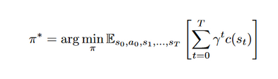
where the expectation is taken with respect to the joint distribution over the sequence of states and actions, often referred to as a trajectory, which has the density

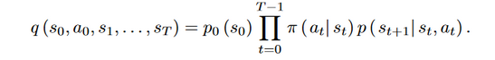
This problem of finding the cost-minimizing policy is known as the policy search problem. To enable generalization to unseen states, the policy is typically parameterized and minimization is performed over representable policies. Solving this problem exactly is intractable in all but selected special cases. Therefore, policy search methods generally tackle this problem by solving it approximately.In many practical settings,p, which characterizes the dynamics, is unknown and must therefore be estimated. Additionally, because it is often equally important to minimize cost at earlier and later time steps, we will henceforth focus on the undiscounted setting, i.e. the setting where $\gamma$= 1.

Guided policy search is a method for performing policy search in continuous state and action spaces under possibly unknown dynamics. It works by alternating between computing a target distribution over trajectories that is encouraged to minimize cost and agree with the current policy and learning parameters of the policy in a standard supervised fashion so that sample trajectories from executing the policy are close to sample trajectories drawn from the target distribution. The target trajectory distribution is computed by iteratively fitting local time-varying linear and quadratic approximations to the (estimated) dynamics and cost respectively and optimizing over a restricted class of linear-Gaussian policies subject to a trust region constraint, which can be solved efficiently in closed form using a dynamic programming algorithm known as linear-quadratic-Gaussian (LQG).

At the point of writing, we are not aware of any model-based reinforcement learning methods used to find the optimal search space for automatic neural architecture design.

Architecture Search via Tree Based Methods¶

Another alternative approach for finding optimal architectures is also what is sometimes referred as Programming by Demonstration. In these methods, the strategy/policy is based upon inputs and outputs which are recorded at very instance which we do guided search using MCTS or Monte-Carlo Tree Search. Also another popular approach used in Markov Decision Monte Carlo Tree Search.

While highly interpretable, but this approach has multiple limitations. MCTS works by exploring several single method and optimizing for global optimum which can be computationally expensive. This was explored by studying the performance of MCTS methods in the 2013 paper Investigating the Limits of Monte-Carlo Tree Search Methods in Computer Go.

Model Optimization- HPO and Regularization¶

While the progress in the field of AutoML has followed the step-wise progressive direction of from doing effective feature designing to manual tuning of various hyper-parameters and implementing regularization techniques to architecture designing one of the key contributions of this paper is to instead look at the problem of automatic model creation and hyperparameter tuning in a top-down fashion instead of a bottom-up approach that explores various hacks to produce substantial predictive and computational gains over our datasets. We believe that the problem of automatic model generation lies at the heart of AutoML and other various optimization techniques can instead be used to further the performance of such automatically generated models. One of the key advantages of this approach is the focus on general-use architectures that can adapt well to non-stationary and cross-domain data i.e. transfer learning. In the past two years, transfer learning has managed to effectively adapt to new domains including in Video Classification to Sentiment Analysis in NLP. The biggest advantage of adopting this line of thinking is the idea of reducing human time and effort required in creating ML model pipelines that lies at the heart of AutoML. We believe the bottom-up approach is rather contrarian in increasing the amount of manual human effort and computational efforts required in testing various approaches since designing architectures still requires a lot of expert knowledge and takes ample time.

Various ways in which the performance of state-of-the-art architectures can be improved includes inclusion of more diverse data for training, or trying various possibly architectures, both being expensive tasks. In order to reduce model overfitting, regularization is used to penalize the model loss for complex models. The basic intuition is that smaller magnitude of model weights will produce a simpler model, thereby reducing overfitting. Normalization techniques can fasten the training process of deep neural networks. The input distribution for each layer in a network changes with updation in parameters of the previous layer, referred to as Internal Covariance Shift. Batch Normalization reduces this shift by taking mean and variance of each layer as a constant, and integrating normalization in the neural network architecture, thereby accelerating the end-to-end training process. The dependency if gradients on input values and scale is considerably reduced, allowing larger learning rates. It also acts as a regularizer, reducing the need of Dropout. However, simply normalizing inputs of each layer can change the meaning represented by each layer. This is tackled by introducing parameters which scale and shift each activation, and learnt during the training process. Secondly, this model uses mini-batches of the training dataset to estimate mean and variances. Weight Normalization, on the other hand aims to reparametrize weight vectors into a parameterized vector and a scalar parameter, in such a way that the Euclidean norm of the weight vector is equal to the scalar parameter. Thus acceleration in the training process can be attributed to decoupling the weight vector’s norm from its direction. Weight normalization reduces the required overheads and is not dependent on batch size.

Another way could be to find the optimal values of hyperparameters in the hyperparameter space which minimizes the loss. The naive approach is to incorporate grid search, which evaluates all possible combinations of hyperparameters. However, this isn’t feasible in real-time, because hyperparameter space is multi-dimensional with infinitely many possible values for the numerical hyperparameters. The next step to perform random search which tests random combinations of hyperparameters within the limits of resources or until a desirable performance is achieved. The success of random search lies in the fact that there are only a few hyperparameters which affect the model accuracy, thereby reducing the apparent dimensionality of the search space. However, the importance of hyperparameters isn’t known beforehand. The next step, intuitively, is to learn the impact of the hyperparameters and accordingly pay attention to those. Bayesian Optimization, thus builds a probabilistic loss-model, updating it sequentially with the newer combinations being tried out, which are selected by the acquisition function. Other sequential model based algorithms employs Tree Parzen Estimators and Random Forests.

However these approaches lack a method of early termination for poorly performing hyperparameter combinations. Bertrand H. et. al. proposed an approach to fine tune hyperparameters for a machine learning model using an ensemble of two complementary approaches - Bayesian Optimization and Hyperband. Hyperband selects and trains a range of models in the hyperparameter domain, while removing the models with the worst performing models after a certain time spent in training. This step is repeated until only a few combinations are left. Bayesian Optimization invests time on training bad models, while Hyperband doesn’t result in improvement in the quality of selected model with time. Combining these two approaches can overcome both of these problems. Initial configurations are selected uniformly and evaluated using Hyperband, after which subsequent selections are a result of training Gaussian Process. After this, the next set of configurations is sampled from the probability distribution resulting from the normalized expected improvement of un-evaluated configurations.

An alternative approach to hyperparameter optimization is to use gradient based approaches. It uses two contrasting approaches to calculate hypergradient in Reverse and Forward Mode. In the reverse mode formulation, the computation is similar to that of backpropagation through time. The forward mode of hypergradient computation relies on chain rule for computing derivative in order to compute the gradient w.r.t hyperparameters. Forward mode calculation is particularly efficient when the hyperparameter space is much smaller than that of the parameters. In another approach, we aim to overcome the constraint of limited memory when computing gradient w.r.t hyperparameters while optimizing the same on validation set. This is achieved by a procedure which is exactly the reverse of stochastic gradient descent with momentum, which allows to compute gradient of the function of the final trained weights w.r.t. learning rate, initial weight configuration, momentum schedule and any other hyperparameter which may be involved with the time complexity equal to that of forward SGD. However, because of finite precision, this computation results in loss of important information as momentum schedule $\gamma < 1$, therefore discarding bits at every multiplication step. This can be overcome by saving the discarded information at each step, and with $\gamma = 0.9$, less than one bit per average needs to be stored.

Pipeline Optimization for AutoML¶

While machine learning is devised to become a tool that could generate classifications or predictions directly from the data itself however as of now deploying these machine learning models end-to-end is still a challenge that’s currently tackled in part with a lot of intervention from humans at various stages. The key steps in training a machine learning algorithm range from pre-processing to feature selection to prediction.

While still an unsolved problem but in 2016, TPOT was created as an automated pipeline design optimization method for AutoML. TPOT works as an architecture with three kinds of operators where each operator corresponds to a machine learning algorithm. Multiple copies of the entire dataset enter the pipeline for analysis. These various copies are then passed over to various types of feature processing operators are available in TPOT including StandardScalar, RobustScalar, RandomizedPCA, Polynomial Features etc that modify the dataset in some way thus returning the modified dataset. Later, these all features from multiple copies are then combined and best features are selected via Feature Selection Operators including SelectKBest, SelectFwe, Recursive Feature Elimination etc. The goal of this step is to reduce the number of features so as pick only the best features. However, this can also cause leaks and overfitting in automated pipelines. Finally, the selected features are sent to Supervised Classification Operators that include Decision Tree, Random Forest, Extreme Gradient Boosting (XGBoost), Logistic Regression and K-Nearest Neighbour Classifier(KNN) which stores the classifier's predictions as a new feature as well as produce classifications for the pipeline.

PROBLEMS AND CHALLENGES in AutoML¶

Cost Sensitivity¶

Building an AutoML system that looks for all the variations of hyperparameter settings, all learning policies can be a very costly endeavour. Also, this does not favour how natural intelligence works.

Argument 1: During meta-learning, the model is trained to learn tasks in the meta-training set. There are two optimizations at play – the learner, which learns new tasks, and the meta-learner, which trains the learner. Methods for meta-learning have typically fallen into one of three categories: recurrent models, metric learning and learning optimizers.

Model Based Methods¶

The basic idea behind model based methods is fast learning through rapid parameter updation. One way is to feed the input sequentially to a recurrent model which learns the sequence representation to adapt to newer tasks. These RNN models ingest their own weights as additional inputs to identify their errors and update their own weights for better generalization on newer tasks.

Memory Augmented Neural Networks are a family of architectures which learn how to quickly encode previously unseen information and thus learn new tasks after seeing limited samples. A Neural Turing Machine combines a controller with external storage buffer and learns to perform read and write operations in memory using soft attention. The label for an input was presented with an offset of 1 timestamp, which allowed the network to learn to keep the data in memory until the label is presented later and retrieval of earlier information for making predictions. The reading mechanism incorporates content similarity where the cosine similarity between the input feature and the memory rows is computed to produce a read vector which is the weighted sum of memory rows. For the write operation, Least Recently Used Access (LRUA) writer is designed in which the write weight vector is an interpolation between previous least used weight vector and previous read weight vector. The intuition lies in the idea of preserving frequently used information and the fact that recently retrieved information won’t be used again for a while.

MetaNets are used for rapid generalization across various tasks. One neural network is used to predict weights of another neural network and these weights are known as fast weights. Weights learnt using stochastic gradient descent, on the other hand are termed as slow weights. MetaNets combine slow and fast weights. MetaNets consist of an embedding function for learning the input representation and a base learner model which performs the actual learning task. A LSTM network is then used to learn the fast weights for embedding function and a neural network is incorporated to learn the fast weights for base learner from their loss gradients. Thus, here we can see that MetaNets effectively have to learn 4 sets of model parameters.

Thus model based methods effectively design a fast learning mechanism, where the models rapidly update their parameters using their own architecture or by incorporating additional meta learning model.

Metric Learning¶

The metric learning based approaches are analogous to kernel density estimation and nearest neighbours estimation, where the predicted probability for an output label for a data point is equal to the weighted sum of labels for other data points in training sample, where the weight signifies the similarity between the 2 samples.

Koch, Zemel & Salakhutdinov used Siamese Networks to learn embeddings for a pair of images to check if they belong to the same output class. The advantage of this approach lies in its ability to measure similarity between images of unknown classes, but its utility decreases with divergence in tasks from the original training perspective.

Relation Networks are similar to Siamese networks but they captured the correlation between an image and support set by incorporating a CNN classifier rather than using a distance metric. It also used MSE Loss in place of cross entropy, because intuitively, it outputs a relationship score, rather than a classification label.

In another approach - Matching Networks, incorporated attention networks which measured cosine similarity between the embedding for a test sample and corresponding support set images. Since the performance of Matching Networks depends upon the quality of the embeddings learnt, a Bidirectional LSTM was trained over the entire support set for a class label to learn the embeddings. For the test sample, an LSTM incorporating attention with the support set as hidden state was used to learn effective embeddings.

Prototypical Networks learns a prototype feature vector for each class, which is defined as mean over feature vectors learnt for each sample in the support set. For a test sample, the output class can be found by taking softmax over inverse-distances with the prototype vectors.

The major task, therefore, in Metric based methods, is therefore to learn the kernel function, which in turn depends upon learning the embedding function for the test sample and the samples in support set.

Optimization Based Learning¶

Gradient based methods aren’t suitable for learning from a small training dataset or converging in a few steps. One idea is to use an additional meta learner to update the weights of the model at hand in a small number of steps. An LSTM Meta Learning provides the following advantages:

Similarity between cell state update and gradient based update
Analogy between storing history of gradients in momentum based update and memory in LSTM
Parameter sharing across coordinates is incorporated to compress the parameter space for the meta learner

In Model Agnostic Meta-Learning, the parameters for the new task are calculated by performing a single or multiple gradient descent operations on the original parameters. The original model parameters are then updated using stochastic gradient descent using the loss over new parameters for the new problems sampled from a distribution of tasks. The basic idea behind this approach is to learn features which are applicable to a distribution of tasks, rather than to that of a single task.

Meta Learning Approaches, therefore aim at increasing the generalization of a model across tasks, without re-training the entire network, and therefore reducing the cost of learning. Model Based Methods utilize inherent or additional memory for fast updation of model parameters. Metric Learning, on the other hand rely majorly on effective representation learning. Optimization Methods replace gradient based methods to generalize the model across tasks with a smaller dataset in hand or in a fewer number of steps.

Curse of Dimensionality¶

Curse of Dimensionality refers to the problem of exponentially increasing data configurations with a linear increase in dimensions. The statistical challenge lies in the small number of available training tuples available compared to the large number of possible configurations. With increasing dimensions, there is a possibility for the lack of training examples for a given configuration of dimensional values. Machine Learning Algorithms using the nearest neighbour information to perform a task will fail in such a case. Natural intelligence is multidimensional (Gardner, 2011) and given the complexity of the world, generalized artificial intelligence will necessarily be multi-dimensional as well.

The most important property of deep learning is that deep neural networks can automatically find compact low-dimensional representations(features) of high-dimensional data (e.g., images, text and audio). Through crafting inductive biases into neural network architectures, particularly that of hierarchical representations,machine learning practitioners have made effective progress in addressing the curse of dimensionality [Yoshua Bengio, Aaron Courville, and Pascal Vincent. Representation Learning: A Review and New Perspective]

Principal Component Analysis, the most commonly used dimensionality reduction technique maps the data to a lower dimension, such that the resulting variance of the data is maximized. The basic objective is to capture most of the variance in the original data, while reducing the number of dimensions used to represent it. Autoencoders can also be used to perform dimensionality reduction, where they learn a reduced representation in the reduction phase, and then goes on to reconstruct the original data tuple in the reconstruction phase.

Interpretability¶

Deep neural networks tend to perform better than the shallow networks, but is it certain that the improved performance can be attributed to the increased depth of a network? In a related paper, the authors mimicked deep networks with shallow ones by training shallow networks not on the original labels, but on the ones predicted by the deep network. The authors observed that shallow networks at par with the deep networks on CIFAR-10 image recognition and TIMIT phoneme recognition, allowing us to ponder upon the correlation between the training procedures used and the success of deep neural networks. It also opens up room to come up with novel approaches to train a shallow network more accurately.

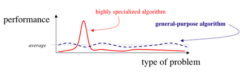
According to the No Free Lunch Theorem for Optimisation:

If an algorithm performs better than random search on some class of problems then in must perform worse than random search on the remaining problems.

In other words, the NFLT states that no black box strategy is superior to another one. Another point to consider is the tradeoff between generality and specificity of an approach.

The need for defining interpretability arises from the gap between objectives in a supervised learning environment and the actual deployment costs. The training procedure only requires the predicted and actual labels for optimization. The problem arises when the real world problem cannot be translated into a mathematical function or because of the difference between the deployment and training settings. Interpretations thus cater to the important but difficult to formalize objectives. The objectives of interpretability are:

Trust: Does the model mimic humans, i.e. performing accurately where humans perform accurately and committing mistakes in areas where humans also struggle? Are we comfortable giving the model the entire control without human supervision?
Causality: Can the associations generated by models be tested experimentally?
Transferability: While supervised learning algorithms are evaluated based upon their performance on the test set, independent of the training data, humans have far more capabilities of generalizing their learnings. This is evident from the failure of machine learning models in adversarial settings.
Informativeness: To provide more information to human decision makers, rather than simply outputting a single value.
Fair and Ethical Decision-Making: Conventional evaluation metrics do not ensure acceptability. Algorithmic decisions must be supported with reasoning and should offer a way to be contested and modified if proven to be wrong.

The paper also expanded on the properties of an interpretable model grouping it under 2 categories:

transparency and
post-hoc explanations.

Transparency: It can be defined at 3 levels:-

At the level of the entire model - Simulatability: Allowing a human to combine input data, along with model parameters and be able to carry out all the computations to produce the output in reasonable time. But how much is “reasonable” amount of time? Are high dimensional linear models, cumbersome rule based systems or huge decision trees interpretable - No. What about a compact neural network?
At the level of individual components - Decomposability: Offering an intuitive explanation to each input, parameter and calculation. Associating descriptions with each node in decision trees or using parameters of a linear model to represent the association strength between features and labels.
At the level of algorithm used - Algorithmic Transparency: A linear model will converge to a unique point even for a new dataset. This however cannot be guaranteed for deep learning mechanisms.

Interpretability: Offer useful information to humans in the form of:

Text Explanations: Train a model to produce an output and a separate model to produce an explanation, mimicking the verbal descriptions of humans.
Visualizations: Qualitatively represent the model’s learnings in form of visualizations.
Local Explanations: Offering local explanations to the decisions of a neural network. A popular example is that of a saliency map which highlights important pixels in an image, which when changed will maximize the effect on the output. In other work, the authors trained a sparse model in locality of a particular point to offer explanation to the decisions of the original model.
Explanation by Examples: Reporting examples which the model consider similar to one under observation. This can be achieved by finding the nearest neighbours in the learned space of the model.

Linear models might seem to be more interpretable than deep learning ones, however they lose simulatability and decomposability with increasing number of dimensions or complexity of features. Deep architectures work on raw features, and thus offer better and more intuitive post-hoc explanations.

Limited Data¶

One of the key arguments here is that humans can learn from very small amount of data. However, deep learning method based AutoML methods and libraries require huge amounts of training data to compute the results. Thus, one of the more apparent limitations of the key AutoML libraries is scenario modelling for the performance of existing models on these particular tasks depend upon the availability of relevant data. This limitation can also be explained by No-Free Lunch Theorem that suggests that no single algorithm can model and provide good predictions on all kinds of data.

One of the methods used in the cases of limited data is probablistic inferencing models that have used to explore compositionality. While compostitional models are yet to match the performance of deep learning based models however one of the AutoML projects developed using this core idea of compositionality is called Automatic Statistician. The main problem for such methods would be computational complexity and the high amount of computational resources required to make predictions. Thus, although theoretically robust, however are also non-scalable.

Linear Regression particularly suffers from lack of data. Relationships learnt from limited data may not portray the accurate trends. For example, the model may learn faster or slower growth in trends than what it actually should be because of lack of sufficient data points.

In the paper Linear Regression with Limited Observation, compared the performance of various regression variants when only a subset of attributes were available. They discovered that while Lasso and Ridge regression required the same number of total attributes to achieve a certain accuracy, SVM Regressors could achieve that with exponentially less attributes.

Many real world scenarios (social media, citation graphs, the Internet etc.) can be visualized in the form of graphs. Two challenges in performing tasks like classification on a graph includes - 1. Absence of labels for many nodes 2. Large computation time for the graph convolutions involved in spectral graph theory. A graph G = (V, E) can be represented using an adjacency matrix A. The input features for the graph can be represented as a N x D matrix, where N are the number of Nodes, and each node had D input features. Each node is associated with an output Z.

Thus, a neural network of the graph G can be summarized as: H(l+1) = f(H(l), A) where input to the first row is the feature matrix and output corresponds to the labels. Kipf & Welling proposed a fast layer wise propagation rule which ensured the inclusion of the feature vector for the node in consideration, as well as normalized the adjacency matrix. The proposed rule is also analogous to differentiable, parameterized form of Weisfeiler-Lehman algorithm, therefore assigning features which captures the role of nodes in the graph. Training this model on a graph, where only a single node is labelled corresponding to each class, the proposed model is able to linearly separate nodes into various classes. The drawback of this approach is the possibility of the proposed approach to underperform on regular graphs.

Missing data poses another problem to learning models which do not overfit the training data. Missing data can be categorized into 3 classes - Missing Completely at Random (MCAR), Missing Not at Random (MNAR) and Missing at Random (MAR). In MAR, the missing data distribution depends on the observed values. MCAR, is a special case where the missing value distribution depends on both observed and missing data. In MNAR, the distribution is independent of observed as well as missing values. Some basic approaches for missing data imputation include Mean Imputation, Gaussian Random Imputation and Expected Maximization Imputation. As their name suggests, Mean Imputation replaces the missing value of the attribute with the mean of available values and Expected Maximization Imputation estimates the missing variable sum and maximizes their mean and covariance using the estimated sum. Gaussian Random Imputation replaces missing values with $\sigma * z + \nu$ where z is a uniformly distributed random standard normal variate and $\sigma$ and $\nu$ are standard deviation and mean of the attribute with missing values. In another work, ensemble methods were used to improve missing value imputation. In Bagging Simple Method, the dataset was resampled and missing values in each dataset was imputed using average of values generated by multiple imputation. After that, a decision tree was constructed for each sample, and their majority vote was used as the classification prediction. In Bagging Multiple Method, an individual decision tree was built for result of each of the dataset generated by multiple imputation. In MI Ensemble, Multiple Imputation is applied on the dataset multiple times, and majority vote of the classifier built on the top of each complete dataset is used. These methods proved to be robust even in scenarios with high percentage of missing data.

For handling image datasets with missing values, variations of GANs and VAEs have been proposed. CollaGAN was proposed which uses a single generator and discriminator network to estimate missing data by looking at the problem of image imputation as multi domain image translation task, and therefore being more memory efficient than other image translation GAN architectures such as CycleGAN.

Comparing the performance of modified Generative Adversarial Networks (GAIN) and Variational Autoencoders for missing data imputation, it is observed that GAIN performs better than VAE for smaller datasets with missing values of numerical attributes but worse on larger ones. VAE tend to be more stable than GAIN, even in cases where they perform worse.

In another approach, the missing values weren’t directly imputed. Instead the missing data was fed to a neural network, and the missing data uncertainty is modeled using probabilistic functions with parametric density, like GMMs, which is learnt with the remaining neural network parameters. Such an approach can work with incomplete datasets, without the need of accurate output for training.

Catastrophic Forgetting¶

Human beings are capable of learning sequentially, where knowledge regarding a new domain doesn't wipe out previously acquired information. Neural Networks, on the other hand, traditionally suffer from a phenomenon called catastrophic forgetting where adaptation over a new task completely wipes out the "memory" of the problem they were previously solving. Lately, there has been some work which promises to overcome catastrophic forgetting and allow networks to learn sequentially.

Intuitively, the most basic way is to keep predictions over old task unchanged when training for newer ones. This, however limits the task distributions. Other way is to ensure that the model parameters always remain in the neighbourhood of optimal parameters achieved for previous iterations. This requires a large number of parameters to be stored. Later, we overcame these disadvantages by training undercomplete autoencoders to preserve feature information important to various tasks.

Deepmind came up with Elastic Weight Consolidation where knowledge is preserved by reducing weight plasticity, where parameter values are drawn back to their older values proportional to their degree of importance for the previous task. EWC, however is sensitive to diagonal approximation of Fischer Information Matrix. Another related work proposed reparametrization of the layers by rotating FIM in the directions which are less prone to forgetting. This resulted in more compact and diagonal FIM.

SupportNet uses SVMs to recognize "support data" which, along with the data for the newer tasks is fed to the neural networks for adapting to newer tasks while retaining information about the older ones. In a related work, the authors used incremental moment matching along with transfer learning techniques like weight transfer and a variant of dropout which boosted the performance of IMM.

Some researchers later used an application oriented view for incremental learning to evaluate the performance of various approaches to cater to catastrophic forgetting. They concluded that dropout doesn't particularly help and EWC, though partly effective still doesn't perform up to the mark.

Towards AGI¶

Current Machine Learning paradigms have achieved human-liker performaces in various domains such as games like Go. However, a very important domain where these models lack the human-like performance is to perform sufficiently well in multiple tasks. Meta Learning, or learning to learn focuses on bridging this gap in Artificial Intelligence. Such models are introduced to numerous tasks, and then they are evaluated on how efficiently they can learn a new one.

Meta Learning tasks can be classified into 3 approaches -:

Using RNNs as base learners, where dataset is processed sequentially and using gradient descent to train the meta learner.
Using a meta-learned metric space, where the base learner follows a comparison scheme and meta learner uses gradient descent.
To learn an optimizer which updates the base learner to efficiently learn a new task. Such a meta-learner is usually an RNN, trained using supervised learning or reinforcement learning which remembers how the base learner was previously updated.

In a different approach Model Agnostic Meta Learning, the authors proposed a model and task independent mechanism which tunes a model’s parameters in order to quickly adapt to a new problem statement with the help of few gradient updates. The parameters for the new task are calculated by performing a single or multiple gradient descent operations on the original parameters. The original model parameters are then updated using stochastic gradient descent using the loss over new parameters for the new problems sampled from a distribution of tasks. The basic idea behind this approach is to learn features which are applicable to a distribution of tasks, rather than to that of a single task. In spite of the simplicity of MAML,it outperformed various few-shot image classification benchmarks, and therefore brought us one step closer to building more versatile agents.

While given the advances in GPUs as well as parallel distribution, several systems are now able to not only compute but also infer the results from past training results. However, one of the key limitations of the widely-accepted methods are their lack of causal inference given these models are trained in a model-blind manner. While there have been several model-based approaches been used in reinforcement learning, however their application to AutoML methods yet remains to be seen and compared against that of model-free methods.

One of the key limitations for these methods in AutoML is the ability to capture abstraction in the data. Several approaches in the past have been thus explored to deal with abstraction and hierarchy in the data namely Fuzzy Set Theory, Rough Set Theory and Quotient Space Based Models.

Christoph Molnar emphasized on understanding how a machine learning model comes up with a prediction, in addition to what the prediction was. The basis of this hypothesis lies closely with human curiosity and our quest to find meaning in life. The study is divided into 2 parts - Interpretable Models and Model Agnostic Methods for interpretability.

Linear models like Linear Regression and Logistic Regression are inherently interpretable models. However, these models suffer from dependence on handcrafted non-linearities and lower predictive performance. Other models including Decision Trees, Decision Rules etc. also fall under the category of interpretable models where importance of each feature can be computed. However these models struggle to accurately model linear correlations.

Model agnostic methods focus on developing stand-alone techniques to interpret the results of a machine learning model. The model is treated as a black box, whose parameters, weights or even architecture is unknown. Certain types of agnostic methods try to model the relationship between the features and the output of the ML model. These methods are easily understandable and intuitive to human beings. However, these methods rely on the assumption of independence among the input features, which is not true for many real world scenarios. Another class of methods focuses on the input features. These methods include the study the meaningful but computationally expensive interaction among the features or studying how the model error changes with permutation in the input feature values. The latter method provides a global overview of the model, but is prone to outliers. The third class of model agnostic methods comprise of surrogate models. The global surrogate method uses the predictions of a black box model for the input data to train an inherently interpretable model, which is then used to carry out the interpretability study. The Local Surrogate Method (LIME) generates permuted data samples for the sample of interest, along with the black-box model’s outcomes for these new data points. It then trains an interpretable model over this newly generate dataset where each input sample’s weight is based upon its distance from the original sample. These methods are flexible and can be used over any type of dataset. However the performance of these methods depend upon the choice and performance of the surrogate interpretable models.

Citation¶

  @article{abi2019,
  title = "Problems & Challenges in AutoML",
  author= "Aryan, Abi; Sareen, Shubhi",
  journal = "abiaryan.com"
  year = "2019"
  month = "Mar"
  url = "https://abiaryan.com/posts/automl-problems-2019/"
  }